Using the `plantTracker` `trackSpp()` function
17 February 2022
Source:vignettes/Using_the_plantTracker_trackSpp_function.Rmd
Using_the_plantTracker_trackSpp_function.RmdIntroduction
This vignette gives detailed information about the
trackSpp() function, the main “workhorse” function in the
plantTracker R package. trackSpp() transforms
a data set of annual maps of plant occurrence into a demographic data
set. To accomplish this, the function compares maps across sampling
years and assigns unique identifiers (“trackIDs”) to plants that overlap
from year to year. Plants with the same trackID are assumed to be the
same individual. These trackIDs are then used to assign survival,
growth, recruit status, and age to each individual plant in each
year.
This process is complex and requires certain assumptions, so the
following pages will explain and illustrate the logic of each of these
steps. We recommend you read through this vignette before using
trackSpp() in order to fully understand the assumptions
inherent to the function, and to make sure that you are adjusting the
user-specified arguments correctly.
1 Input data
The required inputs to the trackSpp() function are
explained in detail in Suggested
plantTracker Workflow, Parts 1.1, 1.2, and 2, as well
as the “help” file for this function (which you can access by typing
?trackSpp in the R console). However, I’ll include a short
description of the arguments here:
trackSpp() argument |
description | required? | default? |
|---|---|---|---|
| dat | An sf data frame in which each row has spatial data for an individual observation in one year. | Yes | N/A |
| inv | A named list in which the name of each element of the list is a
quadrat name in dat, and the contents of that list element
is a numeric vector of all of the years in which that quadrat was
actually sampled (not just the years that have data in
dat!) |
Yes | N/A |
| dorm | A single value greater than or equal to 0 indicating the number of
years these species are allowed to go dormant. OR a
data frame with a row for each species in dat, species
names in the “Species” column and a dormancy value in the “dorm”
column. |
Yes | N/A |
| buff | A single value greater than or equal equal to zero, indicating how
far a far a polygon can move from year i to year
i+1 and still be considered the same individual.
OR a data frame with a row for each species present in
dat, species names in the “Species” column, and a
buff value in the “buff” column. |
Yes | N/A |
| clonal | A logical value (TRUE or FALSE) indicating whether a species is
allowed to be clonal or not. OR a data frame with a row
for each species in dat, species names in the “Species”
column, and a clonal value in the “clonal” column. |
Yes | N/A |
| buffGenet | A single value greater than or equal to zero indicating how close
polygons must be to one another in the same year to be grouped as a
genet. OR a data frame with a row for each species in
dat, species names in the “Species” column, and a
buffGenet value in the “buffGenet” column. |
only if clonal = TRUE
|
N/A |
| species/ site/ quad/ year/ geometry | Five separate arguments, each a character string that indicates the
name of the column in dat that contains data for each of
these required data types. No value is required if the column name is
the same as the default. If only one column names is different than the
default, then you only need to supply a value for that argument. |
No | “Species” /“Site” /“Quad” /“Year” /“geometry” |
| aggByGenet | A logical argument (TRUE or FALSE) that determines whether the output will be aggregated by genet. | No | TRUE |
| printMessages | A logical argument (TRUE or FALSE) that determines if the function returns informative messages. | No | TRUE |
| flagSuspects | A logical argument (TRUE or FALSE) that indicates whether “suspect” individuals will be flagged. | No | FALSE |
| shrink | A numeric value. When two consecutive observations have the same
trackID, and the ratio of size_t+1 to size_t is smaller than the value
of shrink, the observation in year_t gets a
TRUE in the “Suspect” column. |
No | 0.10 |
| dormSize | A numeric value. An individual is flagged as “suspect” if it “goes
dormant” and has a size that is less than or equal to the percentile of
the size distribution for this species that is designated by
dormSize
|
No | 0.05 |
Throughout this vignette, we’ll use a smaller subset of the
grasslandData and grasslandInventory data sets
that are included in plantTracker for examples. The subset
of grasslandData will be referred to as dat,
because it is the dat argument in trackSpp().
The subset of grasslandInventory will be referred to as
inv, since it is used for the inv
argument.
Here are the first few rows of the dat data set we’ll be
using:
#> Simple feature collection with 6 features and 6 fields
#> Geometry type: POLYGON
#> Dimension:     XY
#> Bounding box:  xmin: -0.000160084 ymin: 0.4334812 xmax: 0.286985 ymax: 0.9419673
#> CRS:           NA
#>                 Species Type Site Quad Year sp_code_6
#> 1 Heteropogon contortus poly   AZ  SG2 1922    HETCON
#> 2 Heteropogon contortus poly   AZ  SG2 1922    HETCON
#> 3 Heteropogon contortus poly   AZ  SG2 1922    HETCON
#> 4 Heteropogon contortus poly   AZ  SG2 1922    HETCON
#> 5 Heteropogon contortus poly   AZ  SG2 1922    HETCON
#> 6 Heteropogon contortus poly   AZ  SG2 1922    HETCON
#>                         geometry
#> 1 POLYGON ((0.237747 0.908835...
#> 2 POLYGON ((0.2833037 0.85959...
#> 3 POLYGON ((0.008583123 0.449...
#> 4 POLYGON ((0.1480142 0.46983...
#> 5 POLYGON ((0.03573306 0.5259...
#> 6 POLYGON ((0.2441894 0.52689...
Here are the maps for one quadrat in dat over the first
several years of sampling:
#> Warning: Using `size` aesthetic for lines was deprecated in ggplot2 3.4.0.
#> ℹ Please use `linewidth` instead.
#> This warning is displayed once every 8 hours.
#> Call `lifecycle::last_lifecycle_warnings()` to see where this warning was
#> generated.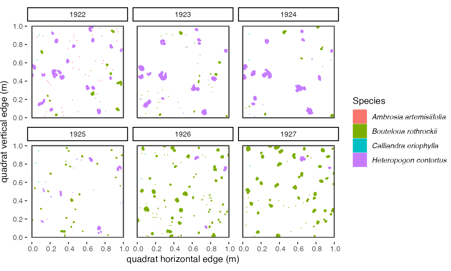
Figure 1.1: Spatial map of a subset of example
dat data set
2 Iterate through sites, quadrats, and species
The first step of trackSpp() is iterating through
dat first by site, then by quadrat, then by species.
inv is also filtered down to a single vector of sequential
sampling years for the quadrat in question. Then trackSpp()
gets the appropriate dorm, clonal,
buff, and buffGenet arguments for that given
species, either by using the globally-specified value in the trackSpp()
function call, or by extracting the species-level value if the argument
was given as a data frame of unique values for each species. Then, the
data and arguments are passed to the assign() function.
This function is not exported in plantTracker, but the code
can be accessed by typing plantTracker:::assign() in the
console. The remainder of this vignette describes the process of the
assign() function.
3 Track individuals over time using the
assign() function
Once the input data has been filtered down to one site, one quadrat,
and one species, then the assign() function is used to
track individuals through time. In this vignette, we will use data from
a site “AZs”, quadrat “SG2”, and the species “Heteropogon
contortus”. The inv vector for this quadrat is
c(1922, 1923, 1924, 1925, 1926, 1927, 1928, 1929, 1930, 1931, 1932, 1933, 1934)
3.1 Get data for the first year of sampling
The data is subset yet again, this time for only the first year of
observations for this species in this quadrat, and stored in a data
frame called tempPreviousYear. In our example, data from
1922 will be stored in this data.frame.
3.2 Group genets together using groupByGenet,
and assign “trackIDs” to each individual in the first year of
sampling
Because this is the first year of sampling, no polygons have been
grouped into genets (if clonal = TRUE), and none have been
assigned trackIDs. Both of these tasks are accomplished by a function
called ifClonal(), which is internal to
assign(). If clonal = FALSE, then clonality is
not allowed, and each polygon is assumed to represent a unique genet. In
this case, each polygon/row in tempPreviousYear is assigned
a unique “genetID” that acts as a temporary identifier that will be used
later in the function.
If clonal = TRUE, then clonality is allowed, and it is
possible for multiple polygons/rows in the raw data to represent one
genetic individual. In this case, we use a function called
groupByGenet() to group polygons together into one genet.
This function uses the buffGenet argument that is supplied
to trackSpp(). The distance (buffGenet x 2) is
the maximum distance that two polygon edges can be from one another and
still be considered ramets from the same genet. In other words, Any two
polygons with edges that are less than (buffGenet x 2) from
one another will get the same “genetID.” groupByGenet()
creates a matrix of distances between every single polygon present in
the input data.frame, and clusters them together based on proximities
that are below the threshold indicated by buffGenet. Then,
basal area is summed for all ramets and stored in the “basalArea_genet”
column of tempPreviousYear. Also, once temporary genetIDs
have been assigned, a permanent “trackID” is given to each genet. This
is a combination of the six letter species code, year of first
observation, and an arbitrary index differentiating individuals of the
the same species and year of recruitment (e.g. HETCON_1922_3).
The following figure shows data for one year (1922) and one species (Heteropogon contortus).
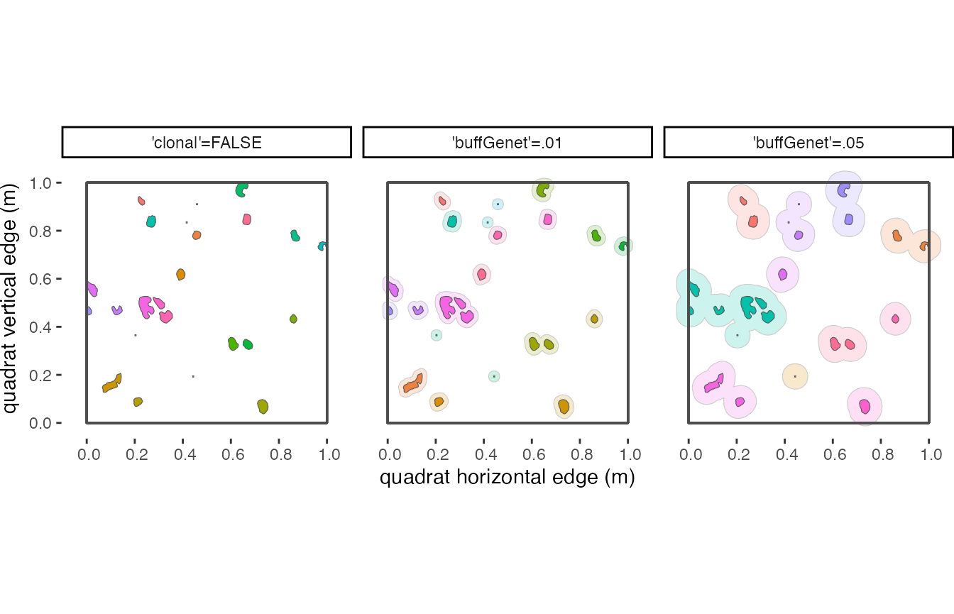
Figure 3.1: The value of ‘buffGenet’ used in the
trackSpp() function can make a big difference in genetID
assignments. These examples move from no genet grouping on the left,
where every polygon has its own genetID, to grouping any ramets together
that are less than 10 cm apart on the right. Colors and numbers indicate
different genetIDs. Buffers are drawn around ramets that belong to the
same genet.
3.3 Assign age and recruitment data to first year
We can also give all individuals in the first year data in the “age”
and “recruit” columns. If the first year for which there is data in
dat is actually the very first year the quadrat was sampled
(e.g. there are Heteropogon contortus observations in 1922, and
the quadrat SG2 was first sampled in 1922), then we put an “NA” in both
the “age” and “recruitment” columns. Because there was no data collected
in the previous year, we don’t know if any of these plants are new
recruits, and don’t know their age.
If the first year of data in dat – now in
tempPreviousYear– is after the first year the
quadrat was sampled (e.g. the first Heteropogon contortus
observations are in 1924, but the quadrat SG2 was first sampled in
1922), then we know that these individuals in
tempPreviousYear really are new recruits and are in their
first year, because they were not present in the previous year. They get
a “1” in both the “recruit” and “age” columns.
If the first year of data in dat is also the
last year that the quadrat is sampled (e.g. the first
Heteropogon contortus observations are in 1934, which is the
last year of sampling), then the observations in
tempPreviousYear get a “1” in both the “recruit” and “age”
columns, but also get an “NA” in the “size_tplus1” and “survives_tplus1”
columns. If this is the case, the assign() function still
uses ifClonal() to assign genetIDs to these observations
and then assigns trackIDs. But there are no further steps needed to
generate demographic data, so the function returns
tempPreviousYear as the result after this point.
3.4 Compare sequential years of data to track individuals through time
Now comes the main work of the function, which compares quadrat maps
for a species over time, and assigns the same trackID to polygons that
overlap from year to year. This is accomplished using a for loop that
compares the previous year of data to the current year of data. The loop
iterates through year by the index i. The “previous” year is
the year with the index i-1 in the inv vector,
and the associated data is stored in the tempPreviousYear
data.frame. The “current” year is the year with the index i in
the inv vector, and the associated data is stored in
tempCurrentYear data.frame. There are multiple if-else
statements nested within this larger for loop, which I’ll explain using
a dichotomous key below.
3.4.1 Is there a gap between year i-1 and year
i?
Not every quadrat was sampled every year, and this is indicated in
the inv vector. This is one case where the
dorm argument input into trackSpp() and then
passed to assign() comes in. The value of dorm
indicates how many years it is “acceptable” for a plant to disappear
from the quadrat maps and still be considered the same individual with
the same trackID. The value of dorm must be determined by
the user, and represents a point where it’s necessary to have some
biological knowledge about the species present in the data set. For
example, allowing dormancy makes sense for some species such as
perennial forbs, but doesn’t for large organisms such as trees.
trackSpp() allows you to specify the dorm
argument globally with one value, or individually for each species. The
dorm argument can also be a way to control how “forgiving”
you want to be with the data set. For example, if you expect that plants
were sometimes missed during the mapping or digitization process, then
allowing a dormancy value of “1” will help account for this. It’s
important to realize that using a dorm value of “1” or
higher will likely slightly overestimate growth and survival,
while using a value of “0” will likely slightly underestimate growth and
survival.
If a gap between inv[i] and inv[i-1]
is… |
|
|---|---|
… greater than the dorm value + 1 (e.g. if
dorm = 1, inv[i] = 1923, and inv[i-1] = 1920; 1923 - 1920
> (1+1)), then we don’t know if the observations in
tempPreviousYear survived or grew. They get an “NA” in the
“size_tplus1” and “survives_tplus1” columns ………. |
Go to step 3.4.11 |
… less than or equal to the dorm value + 1 (e.g. if
dorm = 1, inv[i] = 1923, and inv[i-1] = 1921; 1923 - 1921 =
(1+1)), then we can compare the data from year inv[i-1]
(tempPreviousYear) to data from year inv[i]
(tempCurrentYear) ………………………………. |
Proceed to step 3.4.2 |
3.4.2 Get data for year i
We already have data for the “previous” year (inv[i-1])
stored in tempPreviousYear. Now that we know that the gap
between years doesn’t exceed dorm, we can get data from the
“current” year (inv[i]). We do this by subsetting
dat for all observations in year inv[i]. Then,
we use ifClonal() to group closely-grouped polygons into
genets if applicable, and assign genetIDs. This data set is stored in
the tempCurrentYear data.frame. Proceed to step 3.4.3.
3.4.3 Are there any observations in the “previous” year
(inv[i-1])?
Even if a quadrat was sampled in inv[i-1], it is
possible that there weren’t actually any plants there that year.
| If there … | |
|---|---|
… is data in tempPreviousYear…………. |
Proceed to step 3.4.4 |
… is not data in tempPreviousYear…… |
Go to step 3.4.12 |
3.4.4 Add a buffer around the “previous” year data
Now a buffer is added around each polygon in
tempPreviousYear. This data is stored in the
tempPreviousBuff data.frame. This buffer is of the width
specified in the buff argument of trackSpp()
that is passed to assign(). Adding this buffer before
comparing maps from the previous and current years allows for mapping
error and slight movement of plants between years, which is especially
likely for forbs that resprout every year. Proceed to step 3.4.5.
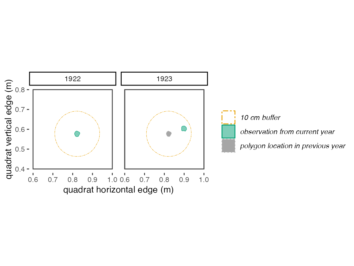
Figure 3.2: With a 10 cm buffer, these polygons in 1922 and 1923 overlap and will be identified by trackSpp() as the same individual and receive the same trackID.
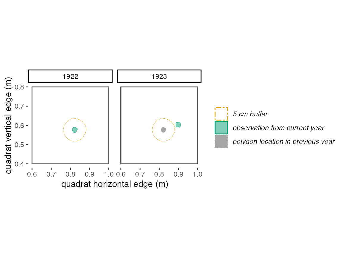
Figure 3.3: With a 5 cm buffer, these polygons in 1922 and 1923 overlap and will be identified by trackSpp() as different individuals and receive different trackIDs.
3.4.5 Are there actually any observations in the “current”
year (inv[i])?
Even if a quadrat was sampled in inv[i], it is possible
that there weren’t actually any plants there that year.
| If there … | |
|---|---|
… is data in tempCurrentYear…………. |
Proceed to step 3.4.7. |
… is not data in tempCurrentYear……. |
Take the entire tempPreviousYear data frame to step 3.4.6
|
3.4.6 Store observations as “ghosts” to compare to data
from the next year (inv[i+1]) during the next iteration of
the loop.
This step also involves the “dormancy” concept discussed in section
[3.4.1]. If dormancy is not allowed for this species
(i.e. dorm = 0), then the observations in question that
were “sent” to this step must be given a “0” in the “survives_tplus1”
column and an “NA” in the “size_tplus1” column. Because they are not
allowed to be dormant, if they don’t have overlapping individuals in the
current year (inv[i])–which they don’t if they’re sent to
this step–then they’re dead. Take these observations to step 3.4.11.
However, if dormancy is allowed for this species, the
individuals that were “sent” to this step because they didn’t overlap
with anything in year inv[i] can be “stored” and compared
to the next set of data from year i+1. We call these stored
individuals “ghosts.” These ghosts will be compared to the polygons from
year i+1, i+2, etc. all the way until the
dormancy argument is exceeded. For example, if some Heteropogon
contortus individuals were present in 1922, but did not overlap
with any plants in 1923 and dorm = 1, then they are stored
as “ghosts” and their locations together with those of individuals from
1923 are compared to the mapped individuals from 1924. If these “ghosts”
have no matches in the 1924 data, then they get a “0” in the
“survives_tplus1” column since they are only allowed to be dormant for
one year. We then call these individuals “dead ghosts.” Any observations
that are sent to this step, but that were observed in a year that is
greater than 1 + dorm years ago, become “dead ghosts.” The
“dead ghosts” are added to the output data.frame. The “ghosts”
are saved for the next step, which is 3.4.12
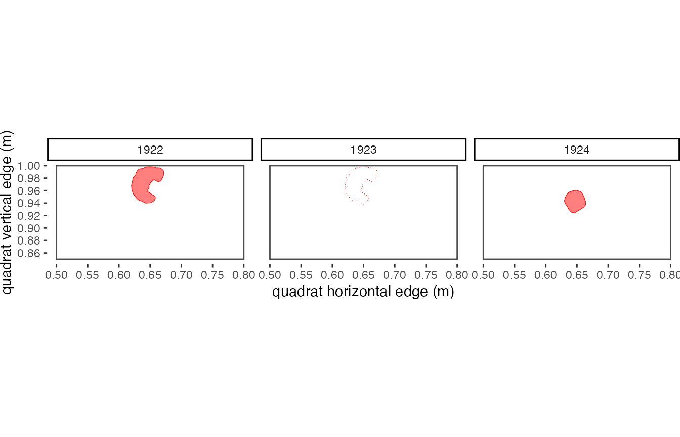
Figure 3.4: A visualization of the ‘dormancy’ scenario described above. The observation in 1922 has no overlap with any observation in 1923 (panels 1 and 2). However, if ‘dorm’ is greater than or equal to 1, we can save the 1922 observation as a ‘ghost’ (illustrated with a dotted border in panel 2). When compared to observations in 1924, there is an overlap! If ‘dorm’ = 1 (or more), then the observation in 1922 will get a ‘1’ in the ‘survives_tplus1’ column. If ‘dorm’ = 0, then the observation in 1922 will get a ‘0’ for survival, and the observation in 1924 will be a new recruit.
3.4.7 Are there any overlaps between polygons in
tempPreviousYear and tempCurrentYear?
Use the st_intersection function from the sf package to
determine if there is any overlap between polygons in the the previous
year (inv[i-1], stored intempPreviousYear) and
the current year (inv[i], stored in
tempCurrentYear).
| If there … | |
|---|---|
… is overlap between tempPreviousYear and
tempCurrentYear……………… |
Proceed to step 3.4.8 |
… is not overlap between tempPreviousYear and
tempCurrentYear… |
Take the tempPreviousYear data frame to step 3.4.6.Take the tempCurrentYear data
frame to step 3.4.12, but first assign them a
“1” in the “recruit” column and a “1” in the “age” column. |
3.4.8 Compare the overlap between
tempPreviousYear and tempCurrentYear to assign
trackIDs.
The st_intersection function used in step 3.4.7 returns a matrix that gives the
total area of overlap between each genet in
tempPreviousYear and each genet in
tempCurrentYear (the “overlap matrix”). There are two
options from here, depending if clonal = TRUE or
FALSE.
If clonal = TRUE, each “parent” (those in
tempPreviousYear) can be represented by more than one
polygon. However, all polygons that are part of the same genet have the
same trackID. “Child” polygons (those in tempCurrentYear)
have not yet been grouped by genet, and do not have trackIDs assigned.
The “overlap matrix” is aggregated by parent trackID so that each parent
trackID has only one row in the matrix. The “overlap matrix” has a
column for each potential child polygon. Each “child” polygon (those in
tempCurrentYear) can have only one parent trackID (but can
have multiple parent polygons). Each “parent” (those in
tempPreviousYear) can have multiple child polygons. In
other words, each row (parent) of the “overlap matrix” is allowed to
have overlap values in more than one column, but each column (child) of
the matrix can only have one overlap value.
If each column of the overlap matrix has only one overlap value, then
the next step is straightforward. Each overlapping “child” polygon is
given the trackID of it’s “parent” in the tempCurrentYear
data frame. If there are multiple “children” that overlap with the same
parent, those children are considered to be ramets of the same genet.
If, however, a “child” overlaps with multiple parents (i.e. a column has
values in more than one row), then we need to determine which potential
“parent” is more likely the true parent. This “tie” is first broken by
comparing the overlap area. The true “parent” is the parent with the
highest degree of overlap with the “child”. In the rare case of a tie
in
overlap area, the parent polygon with a centroid closest to the centroid
of the child polygon is identified as the true “parent”. All other
values in that child column are turned to “NA”s.
If clonal = FALSE, then each “child” can have only one
“parent”, and each “parent” only one “child”. In this case, the
assign() function uses a while loop to look through the
matrix generated by step 3.4.7. The highest value in the matrix
indicates the greatest degree of overlap between a given “parent” and
“child.” The trackID from that parent is given to that child. Then, the
overlap values in the entire “parent” row and “child” columns in the
overlap matrix are changed to zero, since each parent can have only one
child and each child can have only one parent. The while loop repeats
this process of finding the highest value in the matrix to assign
trackIDs until the entire matrix has no non-zero values left.
Take both the tempCurrentYear (child) and
tempPreviousYear (parent) data frames to step 3.4.9.
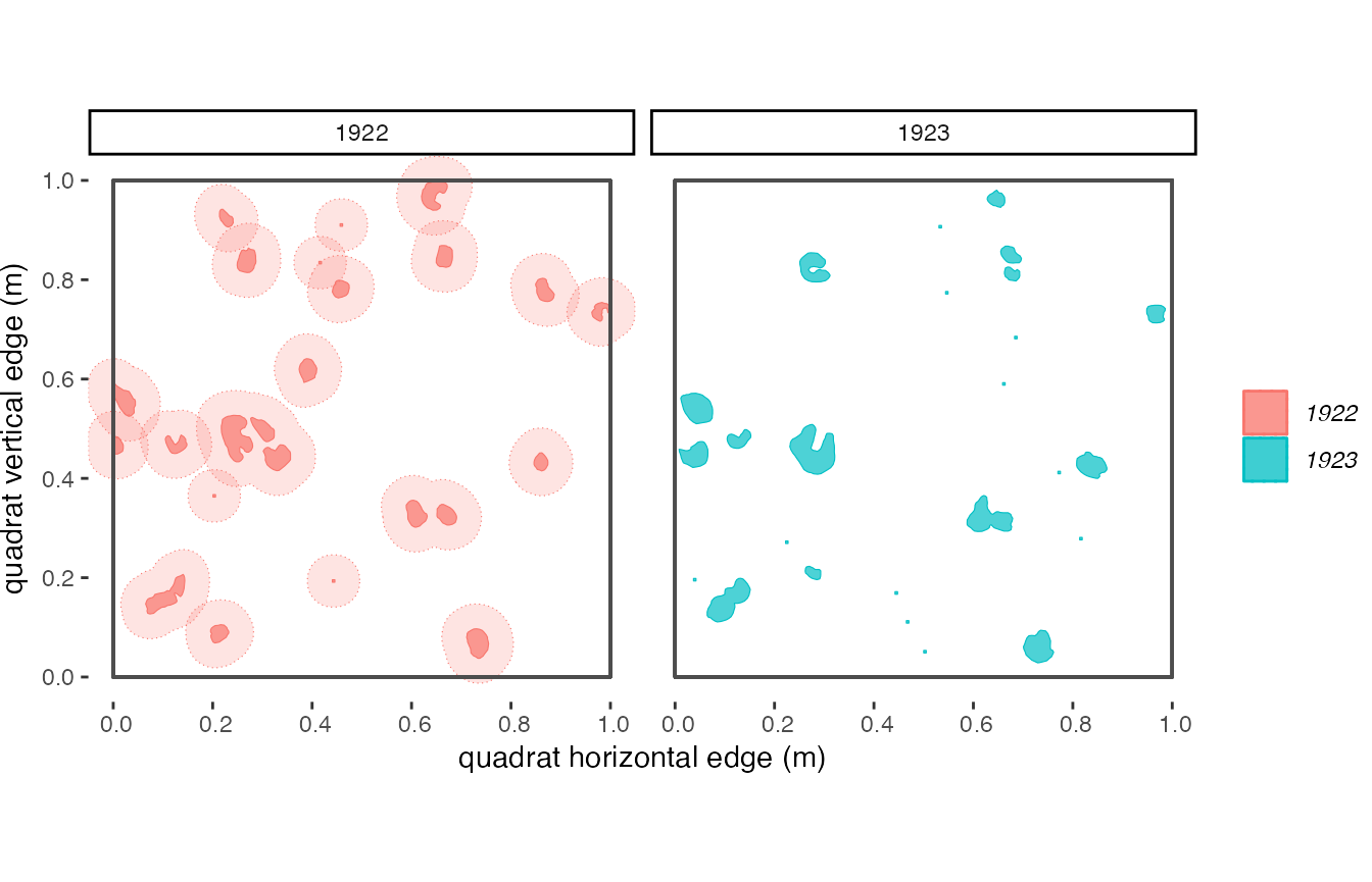
Figure 3.5: Here are the data for Heteropogon contortus* in 1922 and 1923. A 5 cm buffer is shown around each genet in 1922. Data from both years have been grouped by genet using ‘buffGenet’ = .01*
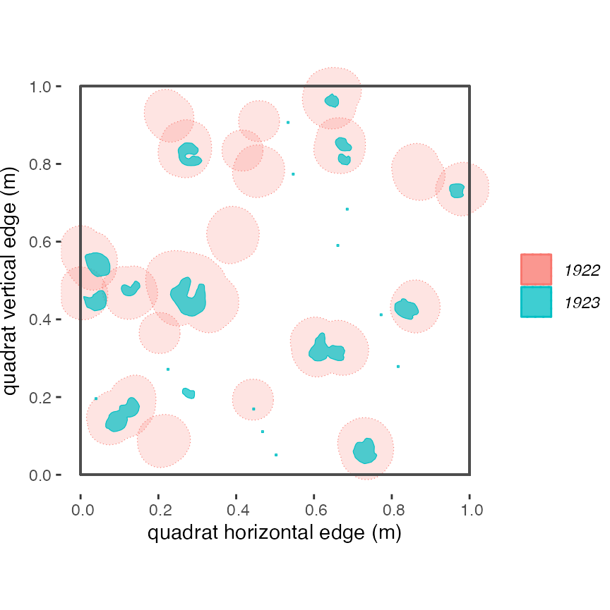
Figure 3.6: Here are the buffered data for Heteropogon contortus from 1922, overlapped with the data from 1923.
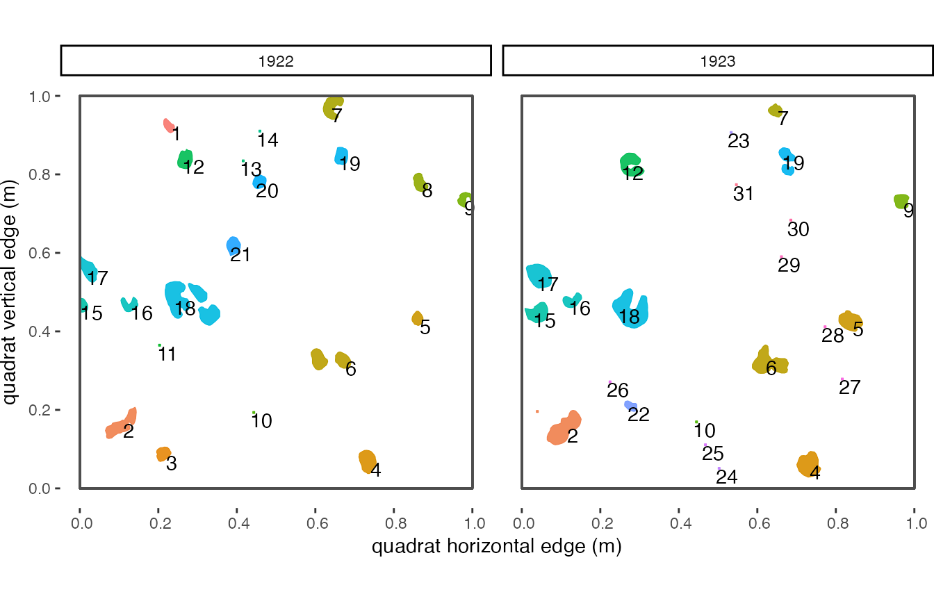
Figure 3.7: Here are the trackID assignments for these two years of data. Each trackID has a different color and a different number.
3.4.9 Flag any suspect observations
If flagSuspects = FALSE, proceed directly to step
3.4.10. If
flagSuspects = TRUE, the following checks take place. The
first check identifies and flags any individuals in the previous year
that became substantially smaller in the current year. For example,
there are two overlapping observations in consecutive years that the
function has given the same trackID. The observation in the previous
year has a basal area of 20 cm\(^2\),
and the observation in the current year has a basal area of 1.5 cm\(^2\). It is possible that these two are in
fact the same individual, but it is also possible that the observation
in the current year is a new recruit that happens to be in a similar
location to the larger plant in the previous year. If
flagSuspects = TRUE, any individual from the previous year
(any “parent”) that has a basal area in the current year below a certain
percentage of its size will be get a “TRUE” in the “Suspect” column.
This threshold is defined by the shrink argument, which has
a default value of 0.10 (10%). To use our previous example, if
shrink = .10, the individual with a basal area of 20
cm\(^2\) in the previous year will be
flagged as “suspect” because it has shrunk to below 10% of its size.
The second check flags very small individuals that go dormant. This
check is only used if the dorm argument is set to “1” or
higher, and if the observations were measured as polygons. This check
can’t be used for observations that were measured as points and
converted to small polygons of a fixed size, since we don’t know the
plant’s true size. A plant with a very small basal area is unlikely to
actually survive dormancy. It is possible that the tracking function has
correctly given the same trackID to a very small individual that is
present in year 1, absent in year 2, and present again in year 3.
However, it is also very possible that this very small individual died,
and the observation in year 3 is a new recruit. This check puts a
TRUE in the “suspect” column of any “parent” individual
that “survives” dormancy if it is below a certain percentile of the size
distribution for that species (which is created using the size data for
that species provided in dat). The percentile threshold is
defined by the dormSize argument, which has a default value
of 0.05 (5%).
Once these checks are complete, the tempCurrentYear
(child) and tempPreviousYear (parent) data frames go to
step 3.4.10.
It is important to note that, even though these checks flag
individuals whose trackID assignment might be “suspect”, the
trackSpp() function still proceeds as it would if
flagSuspects was set to FALSE. It is up to the
user whether they want to exclude “suspect” observations from subsequent
analyses. If you do not exclude these observations, it is possible that
you would slightly overestimate survival, and underestimate recruitment
and growth.
3.4.10 Separate the “ghosts” and the new recruits from the “parent” and “child” data frames
At this point, thetempPreviousYear data frame gets broken
into a parents data.frame, which contains data for all
those genets that have a “child” in the current year, and a
ghosts data.frame, which contains data for those genets
that do not have a “child.” The tempCurrentYear data frame
is broken into a children data.frame, containing the data
for all those genets that have a “parent” in the previous year, and an
orphans data.frame, which contains the data for genets that
do not have a parent.
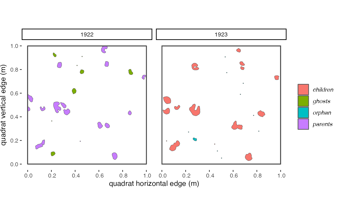
Figure 3.8: Here is a visualization of how the observations are broken into ‘parents’, ‘ghosts’, ‘children’, and ‘orphans’.
The ghosts data frame is sent to step 3.4.6. All of the observations in the
parents data frame get a “1” in the “survives_tplus1”
column, and the total genet area of their “child” is put into the
“size_tplus1” column. Then, the parents data frame
is sent to step 3.4.11 All of the
observations in the children data frame get a “0” in the
“recruit” column, the age column is populated with 1 + the age of their
parent. The observations in the orphans data frame get a
“1” in the “recruit” column and a “1” in the “age” column. However if
the orphans occur after a gap in sampling, they instead get
an “NA” in the “recruit” and “age” columns, since we don’t know whether
they were recruited in year i or during the gap. Then,
both the children and
orphans data.frames are sent to step 3.4.12.
3.4.11 Store the resulting demographic data
Now demographic data (or NAs, if appropriate) and trackIDs have been
assigned to every individual in tempPreviousYear (if there
are actually observations in inv[i-1]), we can save these
results. They are added to a data frame that, when the for loop
finishes, will be returned by the assign() function. If
there are any “dead ghosts”, they are also added to the output
data.frame. If inv[i] is not the last year of
sampling, then proceed to step 3.4.12. If inv[i]
is the last year of sampling, then the for loop is over!
3.4.12 Get ready for the next iteration of the loop
If there are still iterations of the loop left, that is if
inv[i] is not the last year of inv, then the
data from year[i] (stored either in tempCurrentYear or
children and orphans) and any ‘ghosts’ from
previous years are put into the tempPreviousYear
data.frame. This happens even if tempCurrentYear is empty.
If there are not already genetIDs assigned to the data from
inv[i] in tempCurrentYear (which happens if
this is the first year after a gap in sampling), then it is passed
through ifClonal(). The loop proceeds to the next value of
i (start again at section 3.4.1).
Once the loop has progressed through the ‘last’ year, then the output
data set will be saved, and the next species in the data set will be
sent to assign()!
4 Prepare the trackSpp() results to be
returned!
There are just a few more steps in trackSpp() after the
assign() function has been applied to every species present
in the data set.
4.1 Aggregate the results by genet
The data.frames returned by the assign() function are
the exact same length as the input data frames. This means that, even
though trackIDs and demographic data are assigned on the genet level,
each ‘observation’, or ramet, has its own row of data. If the
trackSpp() argument aggByGenet = TRUE, the
output data set is passed through the aggregateByGenet()
function from plantTracker. This aggregates the data set so
that each genet in each year is represented by only one row of data. The
polygons for each ramet are combined into one spatial object using the
st_union function from the sf package. The
resulting data frame will be shorter and narrower than the input
data.frame, since rows are combined. While the output of the
assign() function contains a column for “basalArea_ramet”,
this column is no longer present once the results are aggregated.
If there were any columns in the input data frame beyond those
required (Species, Site, Quad, Year, geometry), these will be dropped
also, since the function can’t predict whether it will be possible to
aggregate those on the genet level. If your input data frame has data in
additional columns that can be aggregated and that you want to keep with
the demographic data, I recommend using aggByGenet = FALSE.
If you want to ultimately aggregate the demographic data by genet, you
can use the sf::aggregate function on your own, or modify
the code for the aggregateByGenet() function to include
your additional columns. If you have set clonal = FALSE for
all species in your input data.frame, I also recommend using
aggByGenet = FALSE, since your results will already be on
the genet scale!
4.2 Informative messages
If the argument printMessages = TRUE, one or two
messages will be printed as each species goes through the
assign() function. These messages are not warnings or
errors! Unless the function returns a message preceded by the word
“warning” or “error”, the function is working! The messages I’m talking
about here provide information about why there are “NA”s present in the
demographic results, which may be concerning if you aren’t expecting
them. The first message tells you which year is the last year of
sampling for this quadrat. Observations in the last year of sampling
will have an “NA” in both the “survives_tplus1” and “size_tplus” columns
because we have no data to determine whether they survived. The second
message only appears if there is a gap in sampling for that quadrat that
exceeds the dorm argument. The message indicates that
observations in the year(s) preceding that gap will have “NA”s in the
“survives_tplus1” “size_tplus1” columns, since we don’t know when they
died. If both printMessages = TRUE and
aggByGenet = TRUE, an additional message will be printed.
This message will warn that the output data frame is shorter and
narrower than the input data.frame, and will explain why that is.
Lastly, if printMessages = TRUE, the
trackSpp() function will print progress messages that
indicate which site is being run the function, then which species, then
which quadrat. This is helpful both to know how far the function has
gotten in your data, and also is helpful if the function errors out. You
can find roughly where the problem in the data is, since you know the
species, quadrat, and site where the function crashed.
If printMessages = FALSE, then no messages will be
returned.
5 Examples
Here are the trackID assignments for 4 years of observations of Heteropogon contortus from a subset of the SG2 quadrat near Tucson, Arizona. ThetrackSpp function here uses
dorm = 1, clonal = TRUE,
buff = 0.05 and buffGenet = 0.01.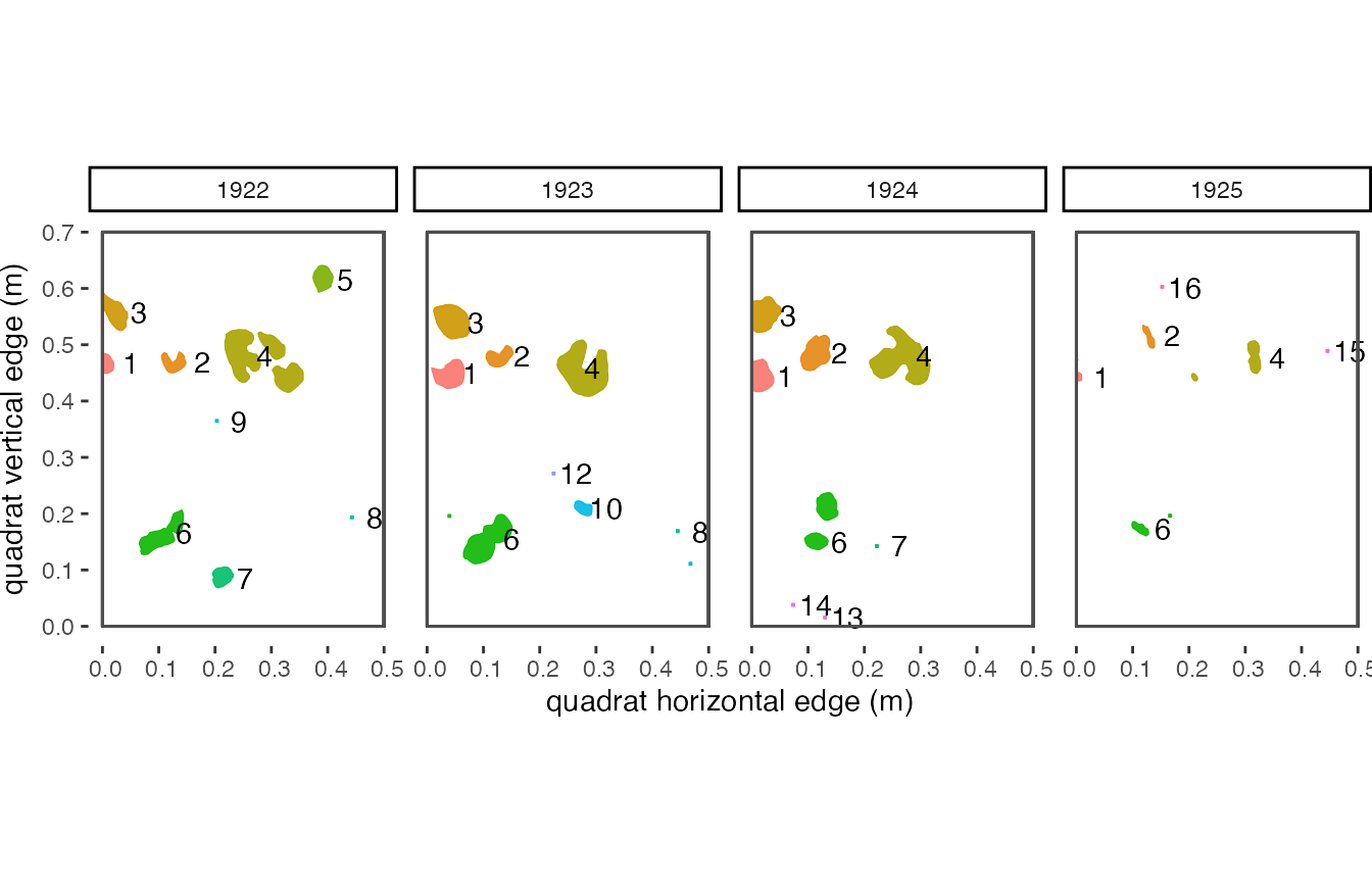
Figure 5.1: Here are the trackID assignments over 4 years of data. Each trackID is shown as a different color and has a different number.
trackSpp()
using a buffGenet value of .05
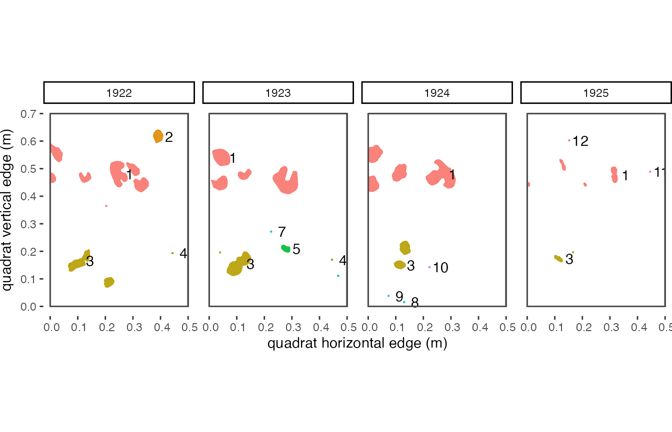
Figure 5.2: Here are the trackID assignments over 4 years of data. Each trackID is shown as a different color and has a different number.
trackSpp() using
clonal = FALSE
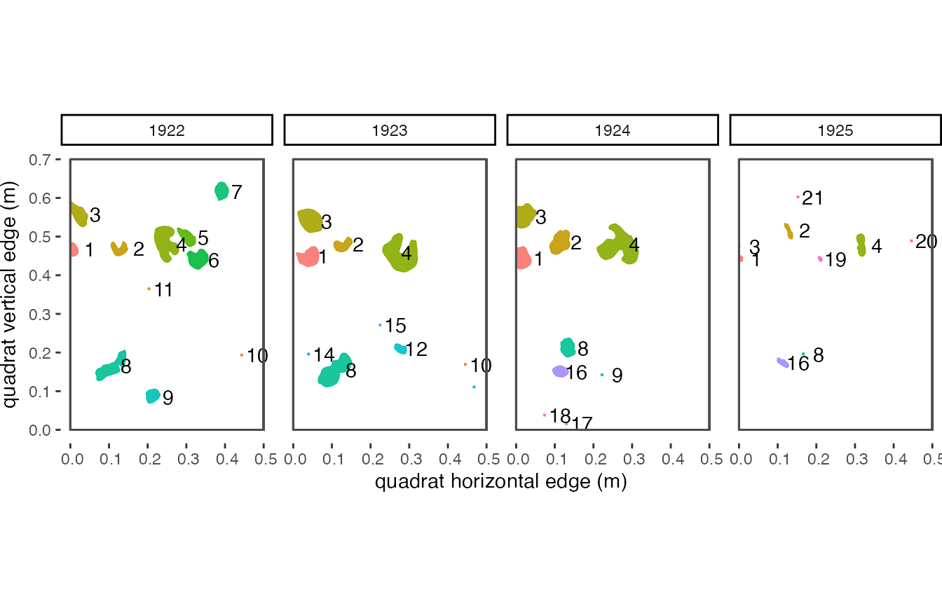
Figure 5.3: Here are the trackID assignments over 4 years of data. Each trackID is shown as a different color and has a different number.